Graph Embeddings: How nodes get mapped to vectors

• Most traditional Machine Learning Algorithms work on numeric vector data
• Graph embeddings unlock the powerful toolbox by learning a mapping from graph structured data to vector representations
• Their fundamental optimization is: Map nodes with similar contexts close in the embedding space
• The context of a node in a graph can be defined using one of two orthogonal approaches - Homophily and Structural Equivalence - or a combination of them
• Once the metrics are defined, the maths are concisely formulated - let's explore.

Graph databases and machine learning

Graph databases enjoy wide enthusiasm and adoption for big data applications of interrelated data from various sources. They are based on a powerful storage concept which enables a concise query language to analyze complex relationship patterns in the data (learn more here). Therefore, algorithms like PageRank, centrality detection, link prediction and pattern recognition can be stated in a simple and intuitive way.

However, most of the well-developed, traditional machine learning algorithms, like linear & logistic regression, neural networks and their alike, work on numeric vector representations. To unlock this powerful toolbox to work on graph structures, we need a way to represent our network of data in a vector form. Graph embeddings are a form of learning exactly this mapping from the data in the graph.

The objective of a graph embedding

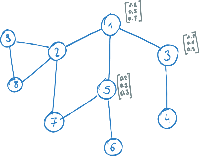
Our goal is to find a vector representation for each node in the graph. Rather than taking into account the associated features of a node, the mapping should represent the network structure of the node. Put differently, the embedding vector of a node should be based on its relationships and neighboring nodes. Nodes which are similar in the graph, should be mapped close in the vector space. The vector space, which we map the node into is called an embedding space.

Now, if we look at the above statement, two questions come to mind, that require additional thought:

• What makes two nodes similar in the graph?
• What does close in the embedding space mean?

Similar nodes in a network

To elaborate on similarity in a graph, let's consider a sentence for a moment:

A sentence is a sequence of words with each word having a definite position. Therefore, a word in a sentence has exactly one ancestor and one successor. To define the context of a word in a sentence, we could use the words surrounding it. For example, the distance-one context of the word 'capital' are the words 'the' and 'of'. The distance-two context would be the words 'is', 'the', 'of', 'Germany'. This is called the n-gram model and is used by a popular approach for finding word embeddings called word2vec.

Similar to n-gram, we can define a context of a node in a graph. Though, we have more choices in a graph structure than in a sequence of words. In general graphs, each node potentially connects to more than two other nodes - whereas in a sentence a word only has one direct ancestor and successor.

Therefore, a sentence is a vector, and a word's context can be explored by moving along the index axis. A graph, however is described as a two-dimensional adjacency matrix, and the direct ancestors of a node is a vector. To explore the context of a node, we have multiple choices at every distance level, and we have to decide how to traverse them.

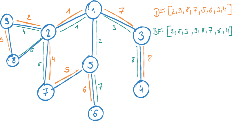
Generally, there are two orthogonal approaches for exploring a network context:

1. Breadth-first: We elaborate on the direct neighbours of our source node first, before we (potentially) move on to the nodes of distance two. This is also called Homophily and is derived from a sociological concept, stating that people generally tend to interact closely with similar others. Therefore, it is based on the assumption that similar nodes in the graph have close relationships.

2. Depth-first: We explore one chain of connections by following a path starting from the source node into its depth first, before we move on to the next. In contrast to Homophily, this metric captures the role of a node in a network from a wider perspective. Rather than looking at close relationships, we seek to find the structural role of a node: e.g. how it is embedded into a larger context of communities. This metric is called Structural Equivalence.

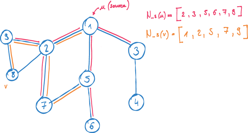
We can use these two approaches to find the context of a node - potentially, by combining them. Having a set of nodes describing the context of each node, we can use these sets to compare each pair of nodes with respect to context similarity. We could apply a Jaccard similarity, for example, to measure how much two contexts overlap. This would give us a way to find nodes with a similar network structure in our graph.

Sampling a context

However, we cannot sample the entire context of any given node as it would eventually lead to capturing the entire graph for any node. Therefore, we employ an approximation which is called a sampling strategy. The idea is to start a fixed amount of random walks in the source vertex to explore its context to generate a random sample. The sampling strategy defined by node2vec combines Homophily and Structural Equivalence. It implements a parameter to decide in each step of the walk whether it should stay close to the source node (Homophily) or should explore another distance level (structural equivalence).

Instead of using the Jaccard similarity described earlier, in node2vec, we try to find a numerical vector for each node. We use the sampled contexts of nodes in the graph, to optimize the mapping function to map nodes with similar contexts close together.

The Maths of node2vec

Let's explore how node2vec works in detail by considering the following example:

V: all nodes in graph
N_S(u): neighborhood of u determined by sample strategy S
f(u): mapping function of node u onto a vector

Our goal is to find embeddings for all nodes u in V, such that the vector representations of nodes with similar contexts are close in the embedding space. We already know what similar contexts in the graph means, but we still need to define, what closeness in the embedding space means.

Let's consider only two nodes in the graph for now:

u: source node
v: node in context of u

To get our maths started, we simply choose two random vectors f(u), f(v) for the two nodes. To measure similarity in the embedding space, we use the dot-product of the two vectors, which is the angle between them.

As node v is in the neighborhood of u, the idea is now to incrementally optimize the mapping function f, such that their similarity gets maximized.

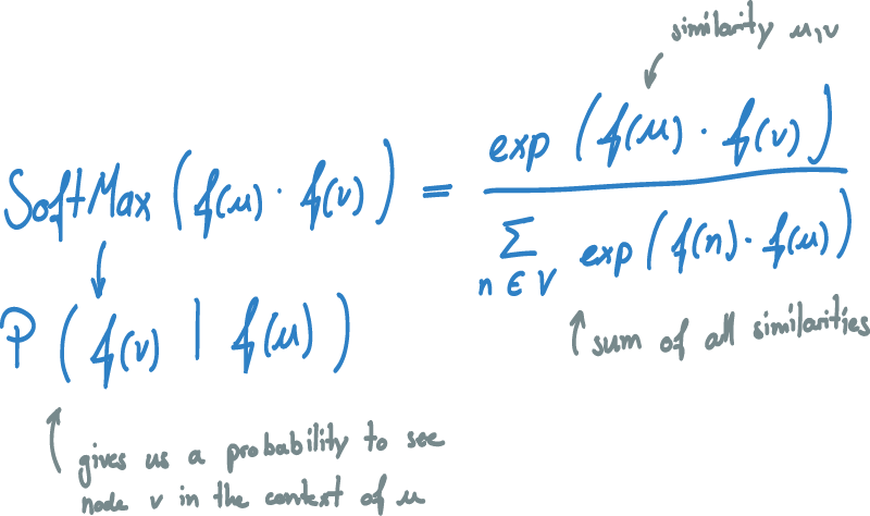
To turn our similarity into a probability, we apply a softmax to it. The softmax normalizes the similarity score dot(f(u), f(v)) with the sum of all similarities of u with all other vectors v in V. The dot-product therefore gets transformed into a number between [0,1] and all similarities add up to a sum of one. The result is the probability of seeing node v in the context of node u from their vector representations. Now, we can incrementally optimize this probability by updating our vector f(u) using Stochastic Gradient Descent.

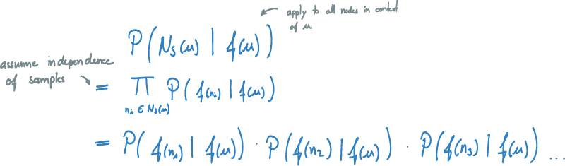
The next step is to generalize this concept to do the optimization not only for one node v in N_S(u), but rather for all nodes in the context of u. We want to optimize the probability of seeing the entire sampled context if we are given node u. If we assume independence of samples, we can simplify this formula into a product of simple probabilities.

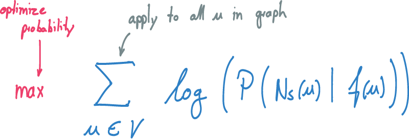
Finally, we want to learn a mapping for each source node u in the graph. Therefore, we apply the formula to all nodes of the graph simultaneously. We optimize the sum using SGD by making adjustments to our mapping f so that the probability increases. We incrementally improve until we reach a maximum number of iterations or find a fixed point in our optimization problem.

Further notes

There is one major challenge when implementing this solution and running it on a large dataset: When we calculate the softmax to determine the probability P(f(v) | f(u)), there is a normalization term in the denominator, which is pretty ugly to calculate. This normalization term is the sum of all similarities of u and all other nodes in the graph. It stays fixed for the entire iteration of the optimization, and therefore also fixed for all iterations of the sum for source node u. The first optimization is to move that factor out of the sum.

The second challenge is that it is very expensive to calculate such a factor over all vectors. In every iteration, we would have to determine the dot-product for every source node u with all other vectors in the graph to find the normalization factor. To overcome this, a technique called negative sampling is used to approximate this factor.

Edge embeddings

The approach described above can also be applied to a different foundational assumption: Instead of finding a mapping of nodes with similar contexts, we could also set a different objective of mapping edges into the embedding space such that these are close, who share same nodes. Combining node and edge embeddings in node2vec, we derive at the more general term graph embeddings, which is capable of mapping interrelated data to vector representations.

Conclusion

We have explored how we can find a mapping f(u) to map nodes of a graph into a vector space, such that similar nodes a close. There are various ways to define similarity of nodes in a graph context: Homophily and Structural Equivalence. Both have orthogonal approaches and node2vec defines a strategy to combine the two into a parameterized sampling strategy. The sampling strategy is a means to find the context of nodes, which is in turn used to derive our embedding. Similarity in the embedding space in turn, is defined as the dot product between the two mapped vectors. The embedding itself is an iterative optimization using Stochastic Gradient Descent. It adjusts the vectors for all nodes in each iteration to maximize the probability of seeing nodes from the same context together. The implementation and application to very large datasets requires some statistical approximation to speed up the calculation.

node2vec is an important key to unlock the powerful tool box of conventional machine learning algorithms to work on graph-structured data.

Me personally, I'm once again taken away by the simplicity and conciseness of the definition of the algorithm to solve the problem at hand. I find it astonishing how well these approaches work if they are applied to the right problem, with the right amount of data.